18: Unstructured meshes with HOHQMesh.jl




Trixi.jl supports numerical approximations on unstructured quadrilateral meshes with the UnstructuredMesh2D mesh type.
The purpose of this tutorial is to demonstrate how to use the UnstructuredMesh2D functionality of Trixi.jl. This begins by running and visualizing an available unstructured quadrilateral mesh example. Then, the tutorial will demonstrate how to conceptualize a problem with curved boundaries, generate a curvilinear mesh using the available software in the Trixi.jl ecosystem, and then run a simulation using Trixi.jl on said mesh.
Unstructured quadrilateral meshes can be made with the High-Order Hex-Quad Mesh (HOHQMesh) generator created and developed by David Kopriva. HOHQMesh is a mesh generator specifically designed for spectral element methods. It provides high-order boundary curve information (needed to accurately set boundary conditions) and elements can be larger (due to the high accuracy of the spatial approximation) compared to traditional finite element mesh generators. For more information about the design and features of HOHQMesh one can refer to its official documentation.
HOHQMesh is incorporated into the Trixi.jl framework via the registered Julia package HOHQMesh.jl. This package provides a Julia wrapper for the HOHQMesh generator that allows users to easily create mesh files without the need to build HOHQMesh from source. To install the HOHQMesh package execute
import Pkg; Pkg.add("HOHQMesh")Now we are ready to generate an unstructured quadrilateral mesh that can be used by Trixi.jl.
Running and visualizing an unstructured simulation
Trixi.jl supports solving hyperbolic problems on several mesh types. There is a default example for this mesh type that can be executed by
using Trixitrixi_include(default_example_unstructured())retcode: Success
Interpolation: 1st order linear
t: 2-element Vector{Float64}:
0.0
3.0
u: 2-element Vector{Vector{Float64}}:
[2.0, 2.0, 2.0, 4.0, 2.0, 2.0, 2.0, 4.0, 2.0, 2.0 … 1.9150968647922513, 3.6675960015371105, 1.9690260025910893, 1.9690260025910893, 1.9690260025910893, 3.8770633988798444, 2.0, 2.0, 2.0, 4.0]
[2.0007938446799503, 1.9996184764271383, 2.0014207716249084, 4.0006477500052835, 2.0017739939500605, 2.0026654709899816, 2.0042560831885705, 4.01412951542216, 2.003418001065543, 2.005769100089331 … 2.088912472670242, 4.351055739867687, 2.034633286662454, 2.0347078235571354, 2.0342991550869214, 4.128372358323666, 2.0037173091210687, 2.0040034762120666, 2.003643980470074, 4.004130908896362]This will compute a smooth, manufactured solution test case for the 2D compressible Euler equations on the curved quadrilateral mesh described in the Trixi.jl documentation. For references on the method of manufactured solutions (MMS) see the following publications:
- Kambiz Salari and Patrick Knupp (2000) Code Verification by the Method of Manufactured Solutions DOI: 10.2172/759450
- Patrick J. Roache (2002) Code Verification by the Method of Manufactured Solutions DOI: 10.1115/1.1436090
Apart from the usual error and timing output provided by the Trixi.jl run, it is useful to visualize and inspect the solution. One option available in the Trixi.jl framework to visualize the solution on unstructured quadrilateral meshes is post-processing the Trixi.jl output file(s) with the Trixi2Vtk tool and plotting them with ParaView.
To convert the HDF5-formatted .h5 output file(s) from Trixi.jl into VTK format execute the following
using Trixi2Vtktrixi2vtk("out/solution_000000180.h5", output_directory = "out")────────────────────────────────────────────────────────────────────────────────────────────────────────────────
Time Allocations
──────────────────────────────── ──────────────────────────────────
Tot / % measured: 675ms / 50.7% 34.1MiB / 61.3%
────────────────────────────────────── ──────────────────────────────── ──────────────────────────────────
Section ncalls time %tot avg alloc %tot avg
────────────────────────────────────────────────────────────────────────────────────────────────────────────────
read data 1 155ms 45.2% 155ms ███▋ 8.19MiB 39.2% 8.19MiB ███▏
read mesh 1 106ms 31.1% 106ms ██▌ 6.44MiB 30.8% 6.44MiB ██▌
add data to VTK file 1 74.2ms 21.7% 74.2ms █▊ 3.44MiB 16.4% 3.44MiB █▍
├─ add data to VTK file 1 123μs 0.0% 123μs 298KiB 1.4% 298KiB ▏
│ └─ element_ids 1 122μs 0.0% 122μs 298KiB 1.4% 298KiB ▏
├─ rho 1 104μs 0.0% 104μs 306KiB 1.4% 306KiB ▏
├─ v1 1 81.9μs 0.0% 81.9μs 298KiB 1.4% 298KiB ▏
├─ v2 1 74.8μs 0.0% 74.8μs 298KiB 1.4% 298KiB ▏
└─ p 1 69.2μs 0.0% 69.2μs 323KiB 1.5% 323KiB ▏
interpolate data 1 5.48ms 1.6% 5.48ms ▏ 301KiB 1.4% 301KiB ▏
build VTK grid (node data) 1 515μs 0.2% 515μs 1.26MiB 6.0% 1.26MiB ▌
build VTK grid (cell data) 1 351μs 0.1% 351μs 1.26MiB 6.0% 1.26MiB ▌
save VTK file 2 225μs 0.1% 112μs 4.98KiB 0.0% 2.49KiB
prepare coordinate information 1 128μs 0.0% 128μs 4.11KiB 0.0% 4.11KiB
prepare VTK cells (node data) 1 9.55μs 0.0% 9.55μs 6.45KiB 0.0% 6.45KiB
prepare VTK cells (cell data) 1 2.10μs 0.0% 2.10μs 6.45KiB 0.0% 6.45KiB
────────────────────────────────────────────────────────────────────────────────────────────────────────────────Note this step takes about 15-30 seconds as the package Trixi2Vtk must be precompiled and executed for the first time in your REPL session. The trixi2vtk command above will convert the solution file at the final time into a .vtu file which can be read in and visualized with ParaView. Optional arguments for trixi2vtk are: (1) Pointing to the output_directory where the new files will be saved; it defaults to the current directory. (2) Specifying a higher number of visualization nodes. For instance, if we want to use 12 uniformly spaced nodes for visualization we can execute
trixi2vtk("out/solution_000000180.h5", output_directory = "out", nvisnodes = 12)────────────────────────────────────────────────────────────────────────────────────────────────────────────────
Time Allocations
──────────────────────────────── ──────────────────────────────────
Tot / % measured: 3.95ms / 78.6% 4.30MiB / 99.8%
────────────────────────────────────── ──────────────────────────────── ──────────────────────────────────
Section ncalls time %tot avg alloc %tot avg
────────────────────────────────────────────────────────────────────────────────────────────────────────────────
build VTK grid (node data) 1 647μs 20.8% 647μs █▋ 1.34MiB 31.3% 1.34MiB ██▌
build VTK grid (cell data) 1 525μs 16.9% 525μs █▍ 1.34MiB 31.3% 1.34MiB ██▌
read data 1 478μs 15.4% 478μs █▎ 25.5KiB 0.6% 25.5KiB
read mesh 1 464μs 14.9% 464μs █▎ 37.6KiB 0.9% 37.6KiB ▏
add data to VTK file 1 457μs 14.7% 457μs █▏ 1.49MiB 34.6% 1.49MiB ██▊
├─ v1 1 118μs 3.8% 118μs ▎ 298KiB 6.8% 298KiB ▌
├─ rho 1 115μs 3.7% 115μs ▎ 298KiB 6.8% 298KiB ▌
├─ v2 1 115μs 3.7% 115μs ▎ 329KiB 7.5% 329KiB ▋
├─ p 1 81.1μs 2.6% 81.1μs ▎ 298KiB 6.8% 298KiB ▌
└─ add data to VTK file 1 19.1μs 0.6% 19.1μs 298KiB 6.8% 298KiB ▌
└─ element_ids 1 18.0μs 0.6% 18.0μs 298KiB 6.8% 298KiB ▌
save VTK file 2 272μs 8.8% 136μs ▊ 4.98KiB 0.1% 2.49KiB
prepare coordinate information 1 178μs 5.7% 178μs ▌ 7.05KiB 0.2% 7.05KiB
interpolate data 1 77.1μs 2.5% 77.1μs ▎ 31.0KiB 0.7% 31.0KiB
prepare VTK cells (node data) 1 6.92μs 0.2% 6.92μs 10.0KiB 0.2% 10.0KiB
prepare VTK cells (cell data) 1 2.46μs 0.1% 2.46μs 10.0KiB 0.2% 10.0KiB
────────────────────────────────────────────────────────────────────────────────────────────────────────────────By default trixi2vtk sets nvisnodes to be the same as the number of nodes specified in the elixir file used to run the simulation.
Finally, if you want to convert all the solution files to VTK execute
trixi2vtk("out/solution_000*.h5", output_directory = "out", nvisnodes = 12)────────────────────────────────────────────────────────────────────────────────────────────────────────────────
Time Allocations
──────────────────────────────── ──────────────────────────────────
Tot / % measured: 72.9ms / 93.0% 82.5MiB / 99.8%
────────────────────────────────────── ──────────────────────────────── ──────────────────────────────────
Section ncalls time %tot avg alloc %tot avg
────────────────────────────────────────────────────────────────────────────────────────────────────────────────
add VTK to PVD file 19 20.5ms 30.3% 1.08ms ██▍ 965KiB 1.1% 50.8KiB ▏
build VTK grid (node data) 19 9.91ms 14.6% 522μs █▏ 25.5MiB 30.9% 1.34MiB ██▌
build VTK grid (cell data) 19 9.22ms 13.6% 485μs █▏ 25.5MiB 30.9% 1.34MiB ██▌
add data to VTK file 19 8.17ms 12.0% 430μs █ 28.2MiB 34.2% 1.48MiB ██▊
├─ v1 19 2.29ms 3.4% 120μs ▎ 5.52MiB 6.7% 298KiB ▌
├─ v2 19 2.25ms 3.3% 118μs ▎ 6.07MiB 7.4% 327KiB ▋
├─ rho 19 1.71ms 2.5% 90.1μs ▎ 5.52MiB 6.7% 298KiB ▌
├─ p 19 1.53ms 2.3% 80.5μs ▏ 5.52MiB 6.7% 298KiB ▌
└─ add data to VTK file 19 334μs 0.5% 17.6μs 5.52MiB 6.7% 298KiB ▌
└─ element_ids 19 327μs 0.5% 17.2μs 5.52MiB 6.7% 298KiB ▌
read data 19 5.44ms 8.0% 286μs ▋ 485KiB 0.6% 25.5KiB
save VTK file 38 4.87ms 7.2% 128μs ▋ 94.7KiB 0.1% 2.49KiB
read mesh 19 4.74ms 7.0% 250μs ▌ 714KiB 0.8% 37.6KiB ▏
prepare coordinate information 19 3.32ms 4.9% 175μs ▍ 134KiB 0.2% 7.05KiB
interpolate data 19 1.31ms 1.9% 68.8μs ▏ 590KiB 0.7% 31.0KiB
save PVD files 2 170μs 0.3% 85.2μs 416B 0.0% 208B
prepare VTK cells (node data) 19 66.7μs 0.1% 3.51μs 189KiB 0.2% 10.0KiB
prepare VTK cells (cell data) 19 38.7μs 0.1% 2.04μs 189KiB 0.2% 10.0KiB
open PVD file 1 22.8μs 0.0% 22.8μs 2.80KiB 0.0% 2.80KiB
────────────────────────────────────────────────────────────────────────────────────────────────────────────────then it is possible to open the .pvd file with ParaView and create a video of the simulation.
Creating a mesh using HOHQMesh
The creation of an unstructured quadrilateral mesh using HOHQMesh.jl is driven by a control file. In this file the user dictates the domain to be meshed, prescribes any desired boundary curvature, the polynomial order of said boundaries, etc. In this tutorial we cover several basic features of the possible control inputs. For a complete discussion on this topic see the HOHQMesh control file documentation.
To begin, we provide a complete control file in this tutorial. After this we give a breakdown of the control file components to explain the chosen parameters.
Suppose we want to create a mesh of a domain with straight sided outer boundaries and a curvilinear "ice cream cone" shaped object at its center.

The associated ice_cream_straight_sides.control file is created below.
open("out/ice_cream_straight_sides.control", "w") do io println(io, raw""" \begin{CONTROL_INPUT} \begin{RUN_PARAMETERS} mesh file name = ice_cream_straight_sides.mesh plot file name = ice_cream_straight_sides.tec stats file name = none mesh file format = ISM-v2 polynomial order = 4 plot file format = skeleton \end{RUN_PARAMETERS} \begin{BACKGROUND_GRID} x0 = [-8.0, -8.0, 0.0] dx = [1.0, 1.0, 0.0] N = [16,16,1] \end{BACKGROUND_GRID} \begin{SPRING_SMOOTHER} smoothing = ON smoothing type = LinearAndCrossBarSpring number of iterations = 25 \end{SPRING_SMOOTHER} \end{CONTROL_INPUT} \begin{MODEL} \begin{INNER_BOUNDARIES} \begin{CHAIN} name = IceCreamCone \begin{END_POINTS_LINE} name = LeftSlant xStart = [-2.0, 1.0, 0.0] xEnd = [ 0.0, -3.0, 0.0] \end{END_POINTS_LINE} \begin{END_POINTS_LINE} name = RightSlant xStart = [ 0.0, -3.0, 0.0] xEnd = [ 2.0, 1.0, 0.0] \end{END_POINTS_LINE} \begin{CIRCULAR_ARC} name = IceCream units = degrees center = [ 0.0, 1.0, 0.0] radius = 2.0 start angle = 0.0 end angle = 180.0 \end{CIRCULAR_ARC} \end{CHAIN} \end{INNER_BOUNDARIES} \end{MODEL} \end{FILE} """) return nothingendThe first three blocks of information are wrapped within a CONTROL_INPUT environment block as they define the core components of the quadrilateral mesh that will be generated.
The first block of information in RUN_PARAMETERS is
\begin{RUN_PARAMETERS}
   mesh file name   = ice_cream_straight_sides.mesh
   plot file name   = ice_cream_straight_sides.tec
   stats file name  = none
   mesh file format = ISM-v2
   polynomial order = 4
   plot file format = skeleton
\end{RUN_PARAMETERS}
The mesh and plot file names will be the files created by HOHQMesh once successfully executed. The stats file name is available if you wish to also save a collection of mesh statistics. For this example it is deactivated. These file names given within RUN_PARAMETERS should match that of the control file, and although this is not required by HOHQMesh, it is a useful style convention. The mesh file format ISM-v2 in the format currently required by Trixi.jl. The polynomial order prescribes the order of an interpolant constructed on the Chebyshev-Gauss-Lobatto nodes that is used to represent any curved boundaries on a particular element. The plot file format of skeleton means that visualizing the plot file will only draw the element boundaries (and no internal nodes). Alternatively, the format can be set to sem to visualize the interior nodes of the approximation as well.
The second block of information in BACKGROUND_GRID is
\begin{BACKGROUND_GRID}
  x0 = [-8.0, -8.0, 0.0]
  dx = [1.0, 1.0, 0.0]
  N  = [16,16,1]
\end{BACKGROUND_GRID}
This lays a grid of Cartesian elements for the domain beginning at the point x0 as its bottom-left corner. The value of dx, which could differ in each direction if desired, controls the step size taken in each Cartesian direction. The values in N set how many Cartesian box elements are set in each coordinate direction. The above parameters define a $16\times 16$ element square mesh on $[-8,8]^2$. Further, this sets up four outer boundaries of the domain that are given the default names: Top, Left, Bottom, Right.
The third block of information in SPRING_SMOOTHER is
\begin{SPRING_SMOOTHER}
   smoothing            = ON
   smoothing type       = LinearAndCrossBarSpring
   number of iterations = 25
\end{SPRING_SMOOTHER}
Once HOHQMesh generates the mesh, a spring-mass-dashpot model is created to smooth the mesh and create "nicer" quadrilateral elements. The default parameters of Hooke's law for the spring-mass-dashpot model have been selected after a fair amount of experimentation across many meshes. If you wish to deactivate this feature you can set smoothing = OFF (or remove this block from the control file).
After the CONTROL_INPUT environment block comes the MODEL environment block. It is here where the user prescribes curved boundary information with either:
- An
OUTER_BOUNDARY(covered in the next section of this tutorial). - One or more
INNER_BOUNDARIES.
There are several options to describe the boundary curve data to HOHQMesh like splines or parametric curves.
For the example ice_cream_straight_sides.control we define three internal boundaries; two straight-sided and one as a circular arc. Within the HOHQMesh control input each curve must be assigned to a CHAIN as shown below in the complete INNER_BOUNDARIES block.
\begin{INNER_BOUNDARIES}

   \begin{CHAIN}
   name = IceCreamCone
   \begin{END_POINTS_LINE}
      name = LeftSlant
      xStart = [-2.0, 1.0, 0.0]
      xEnd   = [ 0.0, -3.0, 0.0]
   \end{END_POINTS_LINE}

   \begin{END_POINTS_LINE}
      name = RightSlant
      xStart = [ 0.0, -3.0, 0.0]
      xEnd   = [ 2.0, 1.0, 0.0]
   \end{END_POINTS_LINE}

   \begin{CIRCULAR_ARC}
      name        = IceCream
      units       = degrees
      center      = [ 0.0, 1.0, 0.0]
      radius      = 2.0
      start angle = 0.0
      end angle   = 180.0
   \end{CIRCULAR_ARC}
   \end{CHAIN}

\end{INNER_BOUNDARIES}
It is important to note there are two name quantities one for the CHAIN and one for the PARAMETRIC_EQUATION_CURVE. The name for the CHAIN is used internally by HOHQMesh, so if you have multiple CHAINs they must be given a unique name. The name for the PARAMETRIC_EQUATION_CURVE will be printed to the appropriate boundaries within the .mesh file produced by HOHQMesh.
We create the mesh file ice_cream_straight_sides.mesh and its associated file for plotting ice_cream_straight_sides.tec by using HOHQMesh.jl's function generate_mesh.
using HOHQMeshcontrol_file = joinpath("out", "ice_cream_straight_sides.control")output = generate_mesh(control_file);The mesh file ice_cream_straight_sides.mesh and its associated file for plotting ice_cream_straight_sides.tec are placed in the out folder. The resulting mesh generated by HOHQMesh.jl is given in the following figure.

We note that Trixi.jl uses the boundary name information from the control file to assign boundary conditions in an elixir file. Therefore, the name should start with a letter and consist only of alphanumeric characters and underscores. Please note that the name will be treated as case sensitive.
Example simulation on ice_cream_straight_sides.mesh
With this newly generated mesh we are ready to run a Trixi.jl simulation on an unstructured quadrilateral mesh. For this we must create a new elixir file.
The elixir file given below creates an initial condition for a uniform background flow state with a free stream Mach number of 0.3. A focus for this part of the tutorial is to specify the boundary conditions and to construct the new mesh from the file that was generated in the previous exercise.
It is straightforward to set the different boundary condition types in an elixir by assigning a particular function to a boundary name inside a Julia dictionary, Dict, variable. Observe that the names of these boundaries match those provided by HOHQMesh either by default, e.g. Bottom, or user assigned, e.g. IceCream. For this problem setup use
- Freestream boundary conditions on the four box edges.
- Free slip wall boundary condition on the interior curved boundaries.
To construct the unstructured quadrilateral mesh from the HOHQMesh file we point to the appropriate location with the variable mesh_file and then feed this into the constructor for the UnstructuredMesh2D type in Trixi.jl
# create the unstructured mesh from your mesh fileusing Triximesh_file = joinpath("out", "ice_cream_straight_sides.mesh")mesh = UnstructuredMesh2D(mesh_file);The complete elixir file for this simulation example is given below.
using OrdinaryDiffEqLowStorageRKusing Trixiequations = CompressibleEulerEquations2D(1.4) # set gas gamma = 1.4# freestream flow state with Ma_inf = 0.3@inline function uniform_flow_state(x, t, equations::CompressibleEulerEquations2D) # set the freestream flow parameters rho_freestream = 1.0 u_freestream = 0.3 p_freestream = inv(equations.gamma) theta = 0.0 # zero angle of attack si, co = sincos(theta) v1 = u_freestream * co v2 = u_freestream * si prim = SVector(rho_freestream, v1, v2, p_freestream) return prim2cons(prim, equations)end# initial conditioninitial_condition = uniform_flow_state# boundary condition typesboundary_condition_uniform_flow = BoundaryConditionDirichlet(uniform_flow_state)# boundary conditions (NamedTuple)boundary_conditions = (; Bottom = boundary_condition_uniform_flow, Top = boundary_condition_uniform_flow, Right = boundary_condition_uniform_flow, Left = boundary_condition_uniform_flow, LeftSlant = boundary_condition_slip_wall, RightSlant = boundary_condition_slip_wall, IceCream = boundary_condition_slip_wall);# DGSEM solver.# 1) polydeg must be >= the polynomial order set in the HOHQMesh control file to guarantee# freestream preservation. As a extra task try setting polydeg=3# 2) VolumeIntegralFluxDifferencing with central volume flux is activated# for dealiasingvolume_flux = flux_ranochasolver = DGSEM(polydeg = 4, surface_flux = flux_hll, volume_integral = VolumeIntegralFluxDifferencing(volume_flux))# create the unstructured mesh from your mesh filemesh_file = joinpath("out", "ice_cream_straight_sides.mesh")mesh = UnstructuredMesh2D(mesh_file)# Create semidiscretization with all spatial discretization-related componentssemi = SemidiscretizationHyperbolic(mesh, equations, initial_condition, solver, boundary_conditions = boundary_conditions)# Create ODE problem from semidiscretization with time span from 0.0 to 2.0tspan = (0.0, 2.0)ode = semidiscretize(semi, tspan)# Create the callbacks to output solution files and adapt the time stepsummary_callback = SummaryCallback()save_solution = SaveSolutionCallback(interval = 10, save_initial_solution = true, save_final_solution = true)stepsize_callback = StepsizeCallback(cfl = 1.0)callbacks = CallbackSet(summary_callback, save_solution, stepsize_callback)# Evolve ODE problem in time using `solve` from OrdinaryDiffEqsol = solve(ode, CarpenterKennedy2N54(williamson_condition = false); dt = 1, # solve needs some value here but it will be overwritten by the stepsize_callback ode_default_options()..., callback = callbacks)retcode: Success
Interpolation: 1st order linear
t: 2-element Vector{Float64}:
0.0
2.0
u: 2-element Vector{Vector{Float64}}:
[1.0, 0.3, 0.0, 1.830714285714286, 1.0, 0.3, 0.0, 1.830714285714286, 1.0, 0.3 … 0.0, 1.830714285714286, 1.0, 0.3, 0.0, 1.830714285714286, 1.0, 0.3, 0.0, 1.830714285714286]
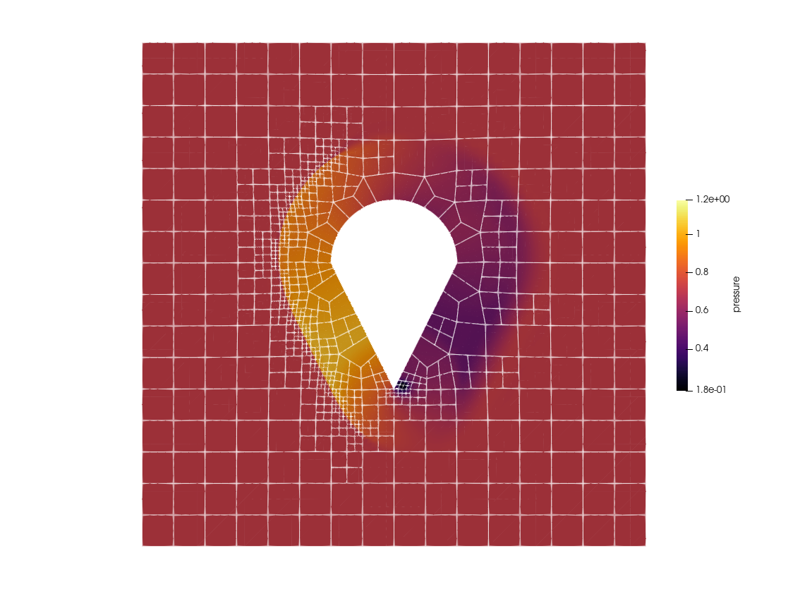
[0.9999999999999996, 0.30000000000000027, 8.305396032730212e-16, 1.8307142857142849, 0.9999999999999993, 0.30000000000000016, 1.4841998707801e-16, 1.8307142857142846, 0.9999999999999996, 0.29999999999999966 … -0.3403500755605527, 2.187243245625583, 1.0467672685115001, 0.22560501375589206, -0.4381435195331212, 2.0641806029671113, 0.9299681196059543, 0.2947198098284334, -0.5408936563796997, 1.883595464663418]Visualization of the solution is carried out in a similar way as above. That is, one converts the .h5 output files with trixi2vtk and then plot the solution in ParaView. An example plot of the pressure at the final time is shown below.

Making a mesh with a curved outer boundary
Let us modify the mesh from the previous task and place a circular outer boundary instead of straight-sided outer boundaries. Note, the "ice cream cone" shape is still placed at the center of the domain.
We create the new control file ice_cream_curved_sides.control file below and will then highlight the major differences compared to ice_cream_straight_sides.control.
open("out/ice_cream_curved_sides.control", "w") do io println(io, raw""" \begin{CONTROL_INPUT} \begin{RUN_PARAMETERS} mesh file name = ice_cream_curved_sides.mesh plot file name = ice_cream_curved_sides.tec stats file name = none mesh file format = ISM-v2 polynomial order = 4 plot file format = skeleton \end{RUN_PARAMETERS} \begin{BACKGROUND_GRID} background grid size = [1.0, 1.0, 0.0] \end{BACKGROUND_GRID} \begin{SPRING_SMOOTHER} smoothing = ON smoothing type = LinearAndCrossBarSpring number of iterations = 25 \end{SPRING_SMOOTHER} \end{CONTROL_INPUT} \begin{MODEL} \begin{OUTER_BOUNDARY} \begin{PARAMETRIC_EQUATION_CURVE} name = OuterCircle xEqn = x(t) = 8.0*sin(2.0*pi*t) yEqn = y(t) = 8.0*cos(2.0*pi*t) zEqn = z(t) = 0.0 \end{PARAMETRIC_EQUATION_CURVE} \end{OUTER_BOUNDARY} \begin{INNER_BOUNDARIES} \begin{CHAIN} name = IceCreamCone \begin{END_POINTS_LINE} name = LeftSlant xStart = [-2.0, 1.0, 0.0] xEnd = [ 0.0, -3.0, 0.0] \end{END_POINTS_LINE} \begin{END_POINTS_LINE} name = RightSlant xStart = [ 0.0, -3.0, 0.0] xEnd = [ 2.0, 1.0, 0.0] \end{END_POINTS_LINE} \begin{CIRCULAR_ARC} name = IceCream units = degrees center = [ 0.0, 1.0, 0.0] radius = 2.0 start angle = 0.0 end angle = 180.0 \end{CIRCULAR_ARC} \end{CHAIN} \end{INNER_BOUNDARIES} \end{MODEL} \end{FILE} """) return nothingendThe first alteration is that we have altered the second block of information BACKGROUND_GRID within the CONTROL_INPUT to be
\begin{BACKGROUND_GRID}
   background grid size = [1.0, 1.0, 0.0]
\end{BACKGROUND_GRID}
This mesh control file has an outer boundary that determines the extent of the domain to be meshed. Therefore, we only need to supply the background grid size to the BACKGROUND_GRID control input.
The second alteration is that the MODEL now contains information for an OUTER_BOUNDARY. In this case it is a circle of radius 8 centered at [0.0, 0.0, 0.0] written as a set of PARAMETRIC_EQUATION_CURVEs.
   \begin{OUTER_BOUNDARY}

      \begin{PARAMETRIC_EQUATION_CURVE}
         name = OuterCircle
         xEqn = x(t) = 8.0*sin(2.0*pi*t)
         yEqn = y(t) = 8.0*cos(2.0*pi*t)
         zEqn = z(t) = 0.0
      \end{PARAMETRIC_EQUATION_CURVE}

   \end{OUTER_BOUNDARY}
Just as with the inner boundary curves, we must assign a name to the OUTER_BOUNDARY. It will be included in the generated .mesh file and is used within the Trixi.jl elixir file to set boundary conditions.
Again, we create the .mesh and .tec files with HOHQMesh.jl's function generate_mesh
control_file = joinpath("out", "ice_cream_curved_sides.control")output = generate_mesh(control_file);The files are placed in the out folder.
The resulting mesh generated by HOHQMesh.jl is given in the following figure.

Running Trixi.jl on ice_cream_curved_sides.mesh
We can reuse much of the elixir file to setup the uniform flow over an ice cream cone from the previous part of this tutorial. The only component of the elixir file that must be changed is the boundary condition NamedTuple because we now have a boundary named OuterCircle instead of four edges of a bounding box.
# boundary conditions (NamedTuple)boundary_conditions = (; OuterCircle = boundary_condition_uniform_flow, LeftSlant = boundary_condition_slip_wall, RightSlant = boundary_condition_slip_wall, IceCream = boundary_condition_slip_wall);Also, we must update the construction of the mesh from our new mesh file ice_cream_curved_sides.mesh that is located in the out folder.
# create the unstructured mesh from your mesh filemesh_file = joinpath("out", "ice_cream_curved_sides.mesh")mesh = UnstructuredMesh2D(mesh_file);We can then post-process the solution file at the final time on the new mesh with Trixi2Vtk and visualize with ParaView.

Setting up a simulation with AMR via P4estMesh
The above explained mesh file format of ISM-V2 only works with UnstructuredMesh2D and so does not support AMR. On the other hand, the mesh type P4estMesh allows AMR. The mesh constructor for the P4estMesh imports an unstructured, conforming mesh from an Abaqus mesh file (.inp).
As described above, the first block of the HOHQMesh control file contains the parameter mesh file format. If you set mesh file format = ABAQUS instead of ISM-V2, HOHQMesh.jl's function generate_mesh creates an Abaqus mesh file .inp.
using HOHQMeshcontrol_file = joinpath("out", "ice_cream_straight_sides.control")output = generate_mesh(control_file);Now, you can create a P4estMesh from your mesh file. It is described in detail in the P4est-based mesh part of the Trixi.jl docs.
using Triximesh_file = joinpath("out", "ice_cream_straight_sides.inp")mesh = P4estMesh{2}(mesh_file)Since P4estMesh supports AMR, we just have to extend the setup from the first example by the standard AMR procedure. For more information about AMR in Trixi.jl, see the matching tutorial.
amr_indicator = IndicatorLöhner(semi, variable=density)amr_controller = ControllerThreeLevel(semi, amr_indicator, base_level=0, med_level =1, med_threshold=0.05, max_level =3, max_threshold=0.1)amr_callback = AMRCallback(semi, amr_controller, interval=5, adapt_initial_condition=true, adapt_initial_condition_only_refine=true)callbacks = CallbackSet(..., amr_callback)We can then post-process the solution file at the final time on the new mesh with Trixi2Vtk and visualize with ParaView, see the appropriate visualization section for details.
Package versions
These results were obtained using the following versions.
using InteractiveUtilsversioninfo()using PkgPkg.status(["Trixi", "OrdinaryDiffEqLowStorageRK", "Plots", "Trixi2Vtk", "HOHQMesh"], mode = PKGMODE_MANIFEST)Julia Version 1.10.12
Commit d93beab124c (2026-08-15 10:29 UTC)
Build Info:
Official https://julialang.org/ release
Platform Info:
OS: Linux (x86_64-linux-gnu)
CPU: 4 × AMD EPYC 9V45 96-Core Processor
WORD_SIZE: 64
LIBM: libopenlibm
LLVM: libLLVM-15.0.7 (ORCJIT, generic)
Threads: 1 default, 0 interactive, 1 GC (on 4 virtual cores)
Environment:
JULIA_PKG_SERVER_REGISTRY_PREFERENCE = eager
Status `~/work/Trixi.jl/Trixi.jl/docs/Manifest.toml`
[e4f4c7b8] HOHQMesh v0.2.15
[b0944070] OrdinaryDiffEqLowStorageRK v3.4.0
[91a5bcdd] Plots v1.41.7
[a7f1ee26] Trixi v0.17.12 `~/work/Trixi.jl/Trixi.jl`
[bc1476a1] Trixi2Vtk v0.3.33This page was generated using Literate.jl.